Comparisons: Borda Count 1

Description of the Borda Count

The most well-known positional voting system is the Borda Count. Voters complete their ranked ballots in exactly the same way as for any other preferential method. Using the candidate-listing ballot approach, each voter puts a '1' against their first preference, '2' against their second one, '3' against their third and so on. Truncation may or may not be permitted so voters are required to express a preference for some or all candidates respectively. If eight candidates compete in a Borda Count election, then 8, 7, 6, 5, 4, 3, 2 & 1 points are awarded for a 1st, 2nd, 3rd, 4th, 5th, 6th, 7th & 8th preference respectively. More generally for N candidates, N points are given for a first preference and one point less for every subsequent drop in rank position down to one point for the least preferred candidate. All the points awarded by voters are then tallied for each candidate and the candidate with the most points wins.

Mathematically, the allocation of points to the ranked preferences form a linear progression of values where the common difference between adjacent values is one point. Note the contrast with CHPV where it is the common ratio between adjacent values that is fixed. For the Borda Count, the actual value of the common difference does not matter so long as it is fixed. Nor does the absolute value of any preference matter. For example, the common difference could be fixed at 1/N points and the lowest preference at zero points. The Borda Count will still produce the identical candidate rankings for the same voter input. For a more detailed and comprehensive description of the Borda Count, please visit the voting system section of Wikipedia or another reference source.

Properties of the Borda Count

As the Borda Count is a genuine positional method, it satisfies all those voting system criteria that any positional system adheres to; namely, the summability, consistency, participation, resolvability and Pareto criteria. Unlike CHPV, it fails the mono-raise-random and mono-sub-top monotonicity criteria but it does however satisfy the reversal symmetry criterion.

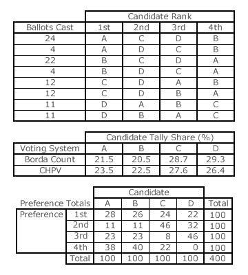
The tables opposite illustrate some other features of the Borda Count. The voter input here is identical to the example election in the preceding section but the election outcome is now determined by the Borda Count instead of FPTP. The winner this time is candidate D despite D having the fewest number of first preferences. The Borda Count does not seek to satisfy the majority criterion.

Indeed, with a large field of candidates, one with first preferences from a huge majority of the voters can still be beaten by another with a second preference from every voter. For example, consider an election with 100 voters and 10 candidates. The candidate with all the second preferences scores 900 points (= 100 x 9). As a first preference is worth 10 points, a winning candidate must get a first preference from over 90 (= 900/10) of the 100 voters to win. Failing to reach this threshold means that the consensus candidate with no first preferences wins. Contrast this with FPTP where this same candidate would receive zero votes!

In the election opposite, the more polarized candidates A and B are ranked above the more consensual candidates C and D when using FPTP (see previous section). Using the Borda Count, note that the consensus candidates are now ranked above the polarized ones. When compared to CHPV, candidate D now overtakes C to win. To understand why D is ranked top refer to the preference totals table opposite.

Notice that candidate D is the least disliked having no fourth (last) preferences at all while A and B have strong opposition to their winning. With 22 first, 32 second, 46 third and no fourth preferences, the average rank position for D is [(22 x 1) + (32 x 2) + (46 x 3) + (0 x 4)]/100 or 2.24. For A, B and C, it is 2.71, 2.77 and 2.28 respectively. The following two properties apply to any Borda Count election where truncation does not occur.

• As an alternative to the descending order of candidates tallies, the ascending order of candidate average rank positions can be used instead to list candidates in collective descending rank order.
• To win, a candidate requires an average rank position that is lowest in value and hence highest in rank.

Therefore, in descending rank order, D at 2.24 is ranked first, C at 2.28 is second, A at 2.71 is third and B at 2.77 is last. In the Borda Count, consensus beats polarization. To win, a candidate must maximise their preference from each and every voter. Persuading a voter to change their support from last to penultimate preference is just as important as changing from second to first. For the Borda Count (or GV with r → 1), it is the average preference that determines the winner. For GV with r = 1/2 (CHPV), it is the above-mean-weighted preferences that matter. For FPTP (or GV with r = 0), only the very top preferences count. The relationship between the key preferences that determine an election outcome and the common ratio employed in GV is explored in greater depth in the later Comparisons: Geometric Voting section.

Proceed to next page > Comparisons: Borda Count 2

Return to previous page > Comparisons: Plurality (FPTP) and Anti-Plurality 2