Comparisons: D'Hondt ~ Proportionality 1

Disproportionality Indices

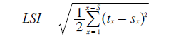
For party-list CHPV, the Gallagher or Least Squares Index (LSI) is employed as a measure of the discrepancy between the party shares of the tallies (t) and the party shares of the seats (s); where 0 ≤ LSI ≤ 1. If necessary, please refer back to the Evaluations: Proportionality of CHPV section. For convenience, the definition of the least squares index for S parties is repeated here; see opposite.

To facilitate a fair comparison with CHPV, the proportionality of D'Hondt is approached in an identical manner. Two LSIs are again employed to assess disproportionality; one for the seat resolution and the other for the voting system itself. The resolution LSI is based on the discrepancies between the centres and the corners or extremes of the domains. These domains relate to those of an optimally proportional voting (OPV) system. For a given number of parties (S) and seats (W), the number and average size of the domains are identical irrespective of the voting system used. Hence, the resolution LSI is almost identical for OPV, CHPV and D'Hondt.

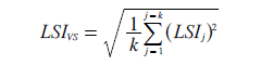
By separating the common discrepancies due to resolution from the unique ones introduced by the voting system itself, a clearer comparison between two rival systems can be achieved. The voting system least squares index (LSI_VS) is also repeated here; see opposite. For a given election (S and W), there are k domains in total and each domain j requires its own LSI to be determined.

The centre of an OPV domain is where perfect party proportionality is achieved between tallies and seats. Like CHPV, the centre of the corresponding D'Hondt domain will be offset from this ideal point. The least squares index for domain j (LSIj) hence measures the disproportionality introduced by the D'Hondt algorithm in offsetting its domain centre. The overall LSI_VS simply combines these individual domain LSIs into one value within, as always, the range 0 ≤ LSI ≤ 1.

D'Hondt Domain Centres

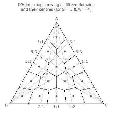
In order to determine the LSI_VS for any particular D'Hondt Party-List election, the position of each domain centre must first be identified. In the example three-party map opposite, all the fifteen domains and their centres for a four-winner election are illustrated.

For the 2:1:1 seat share domain, three two-way tie lines are also shown (as dotted lines) intersecting with each of the three apexes. In each case, the relevant critical sections of the outer pair form two opposing sides of the irregular hexagonal domain. The two-way tie line that intervenes between each outer pair exactly bisects the angle between these two lines. The bisecting lines from the three apexes all intersect at the same point; namely, at the centre of the domain.

The tally shares for the 1:1 tie line are 1/2 and 1/2 for parties A and B when party C has zero. For the 3:1 tie line, they are 3/4 and 1/4 respectively. Hence, for a tie line to bisect the intervening angle, they are required to be respectively 5/8 and 3/8. This bisecting line therefore represents a tally share ratio of A:B = 5:3 as shown. The other two bisecting lines are similarly determined to have ratios of 5:3 for A:C and 1:1 for B:C. The tally share ratio for the 2:1:1 seat share domain centre is hence 5:3:3.

By this method, the centre point of every domain within the three-party map can be established. For two-party maps, the centre of each domain is simply the point of bisection mid-way along its length.

For more than three parties a tabular approach using a general formula for deriving tally shares from seats gained has to be adopted in place of the visual maps. For more details here, please refer to proof CDH1. For S parties competing for W seats, the domain centre tally share (t_Z) for party Z that wins Y_Z seats is given by the following formula.

• t_Z = (Y_Z + 1/2)/(W + S/2)

Note that for perfect proportionality, t_Z = Y_Z/W = s_Z where s_Z is the per-unit share of the seats won by party Z.

Having established the location of every domain centre and the shares of the seats and tallies at each one, the voting system LSI for a D'Hondt method election can then easily be calculated.

Proceed to next page > Comparisons: D'Hondt ~ Proportionality 2

Return to previous page > Comparisons: D'Hondt ~ Party Cloning 2