Comparisons: Party-List ~ Sainte-Laguë

Description of the Sainte-Laguë Method

This method employs the highest averages approach to seat allocation in the party-list voting system as described in the earlier party-list section. For an election with W seats/winners, the Sainte-Laguë divisors are 1, 3, 5, 7 and so on until one less than 2W. In other words, they form a linear sequence of odd integers from 1 to 2W - 1.

Consider the decimal divisors 0.5, 1.5, 2.5 and so on instead. This sequence is the same as the previous D'Hondt divisors (1, 2, 3 and so on) except that they are all 0.5 smaller. This negative offset of one half is designed to reduce the slight bias in favour of the larger parties when using the D'Hondt method. Rather than using these decimal divisors (0.5, 1.5, 2.5 and so on), they are usually all multiplied by two to yield integer ones (1, 3, 5 and so on).

The fact that the integer-divisor averages are half those generated by the decimal ones is irrelevant. The W highest averages still elect the same winners as their rank order is unaffected by the common scaling factor of two. The concept of an absolute 'average' representing a proportion of the voters is distorted by this scaling factor. However, with CHPV and Sainte-Laguë, it is now only the relative size of one 'average' compared to any other that matters in winning seats.

In practice, it is quite common for the first divisor to be 1.4 rather than just 1. This modification is designed to raise the threshold for a small party in gaining its first seat. The analysis of the Sainte-Laguë method in this chapter is based solely on its unmodified version. For a detailed and comprehensive outline description of the Sainte-Laguë Party-List method, please visit the voting system section of Wikipedia or another reference source.

Sainte-Laguë Method Election Example

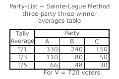
To enable a comparison with all the preceding party-list methods, consider yet again the ongoing three-party three-winner election example but now using the Sainte-Laguë divisors of 1, 3 and 5 to establish the key averages. Parties A, B and C again respectively each receive an 11/24, 8/24 and 5/24 share of the vote. For a nominal total tally of 720 valid votes, the table opposite shows the three candidate averages for each party. The three highest averages are highlighted in white in this table. Therefore, parties A, B and C gain one seat each.

For parties A:B:C, the seat ratio is hence 1:1:1 for the tally ratio of 11:8:5. This outcome is also one of the two tied results (to be resolved by random selection) when using the Droop Quota method; where the other outcome is the non-optimal seat ratio of 2:1:0. The D'Hondt method similarly produces this non-optimal result. The Hare Quota only generates the optimal 1:1:1 outcome. Employing the Sainte-Laguë method here also results in the optimal outcome.

Sainte-Laguë Method Map Construction

Before comparing this method to the party-list CHPV voting system, its own properties must first be established. As with CHPV, issues regarding optimality, party cloning and disproportionality can be addressed once a variety of multiple-party multiple-winner maps have been constructed.

In the following section, the featured two-party and three-party maps for this method are presented without any explanation of their construction. For those advanced visitors to this website who wish to understand how such maps are constructed or who wish to construct ones that are not featured for themselves, then please refer to the Map Construction appendix for either the Two-Party Sainte-Laguë Method Maps or the Three-Party Sainte-Laguë Method Maps page.

Proceed to next section > Comparisons: Sainte-Laguë ~ Maps

Return to previous page > Comparisons: D'Hondt ~ Proportionality 3