Comparisons: Geometric Voting 1

Range of Equivalent Positional Voting Systems

With a variable common ratio (r), GV is able to represent an unlimited range of positional voting systems from first-past-the-post (FPTP) at one extreme (r = 0) to the Borda Count at the other (r → 1). With just two candidates, all voting systems will generate the same outcome as whoever is the more popular wins. Once there are at least three candidates then the differences between the various systems appear in the collective candidate rankings.

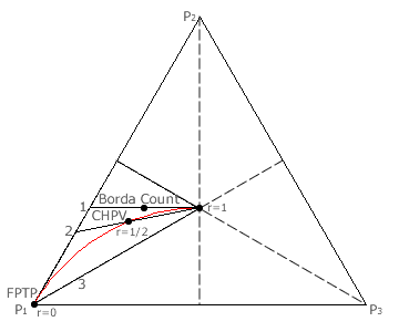
For three candidates in an election using a positional voting system, a three-preference map can be used to define and display the value of the three positional weightings employed in the election; see map opposite. Such maps are very similar in construction and use to the three-party ones introduced in the preceding chapter; see the Three-Party CHPV Maps section for details. Here, each apex of the triangle represents a value of 1 for the stated preference and 0 for the other two. For example, at apex P₁, the first preference has a value of 1 and the second and third ones (P₂ and P₃) have a value of 0. This apex P₁ hence represents the FPTP and GV(r = 0) systems.

The location of CHPV (GV with r = 1/2) is also shown on the map. The weightings plotted on the map are normalised. That is, the three preference values sum to unity; the key property of any triangular map. Therefore, for CHPV, the consecutively halved per-unit weightings are four sevenths, two sevenths and one seventh for P₁, P₂ and P₃ respectively. Each weighting is plotted towards its own apex (w = 1) at right-angles to its opposing baseline (w = 0). For any positional voting system to be legitimate, the first preference must be worth more than the last preference. Also, the lower of two adjacent preferences cannot have a higher weighting. So all systems that lie outside the white area of the map are invalid.

The Borda Count with its usual weightings of three, two and one points is similarly displayed on the map. These three preferences are first normalised to per-unit values of three sixths, two sixths and one sixth before plotting. The GV variant with r → 1 is also shown on the map. Notice that, although they produce equivalent outcomes, these two systems are not synonymous as they generate different tallies; see the Comparisons: Borda Count 3 page. Hence they appear in different locations on the map. With GV (r → 1), both the second and third preference weightings (r and r² respectively) approach a value of one (the weighting of the first preference). The normalised weightings are therefore extremely close to 1/3, 1/3 and 1/3; the centre of the equilateral triangle.

For the Borda Count, the value of the common difference (d) is irrelevant in terms of the collective candidate rankings. Its three normalised weightings are (1 + d)/3, 1/3 and (1 - d)/3. Here, d may validly range between virtually zero (extremely close to the map centre) to one (at the left-hand map edge). So, in fact, all points along a straight line on the map (line 1) represent Borda Count variants with equivalent ranking outcomes.

So far, three GV variants (where r = 0, r = 1/2 and r → 1) are highlighted on the map. When the weightings for continuous values of r between 0 and 1 are evaluated and the locations of the corresponding GV variants are plotted on the map a continuous curve (shown in red) results. This curve is defined below.

• A circular arc from apex P₁ to the map centre (where this end of the arc has a zero gradient) represents the full range of GV variants from r = 0 to r → 1.

Where a common amount is added to each of the three weightings and then a common multiplying factor is used to normalise them, the resultant voting system necessarily produces the same ranking outcomes as the original one in all cases. Equivalent voting systems are easily identified on the map as indicated below.

• Every point on a straight line from map edge to map centre that crosses the arc of GV variants (for example, line 2) represents a voting system that is equivalent to the GV variant represented by the point of intersection.

Consequently, some very important conclusions can now be drawn; as stated below.

• The map region between the Borda Count line (line 1) and the FPTP one (line 3) contains every possible straight line that crosses the arc of GV variants.
• Hence, all possible three-candidate positional voting systems between the Borda Count and FPTP are equivalent in ranking outcomes to that of a GV variant with a common ratio in the range 0 ≤ r < 1.
• Therefore, GV can represent and replace any three-candidate positional voting system between the Borda Count and FPTP by simply adopting the appropriate value for the common ratio.

Proceed to next page > Comparisons: Geometric Voting 2

Return to previous page > Comparisons: Borda Count 3