Comparisons: Positional Voting 1

Description of Positional Voting

Positional Voting encompasses a class of preferential systems employing ranked ballots whereby each rank position (n) is allotted a number of points or weighting (w) consistently across all ballots. The single winner is the candidate receiving the highest tally of weights awarded by the voters. For the distribution of weights to be valid, the following two criteria must be satisfied. Primarily, for any two adjacent preferences, the lower-ranked one must never be worth more than the higher-ranked one; namely w_n+1 ≤ w_n. Secondly, as a system where all the preferences are the same (w₁ = w_n = w_N) is pointless, the first preference must be worth more than the last preference; so w₁ > w_N. For a more detailed and comprehensive description of Positional Voting, please visit the voting system section of Wikipedia or another reference source.

Quantifying Consensus and Polarization Bias within Positional Voting

In order to compare one system against another, it would be useful to develop a suitable index. By rearranging the primary criterion for such systems to become w_n+1/w_n ≤ 1 provided that w_n ≠ 0, a useful index does emerge. This ratio hence represents the relative importance of the lower preference with respect to its adjacent higher one. When both preferences have the same weighting, there is consensus between them and, as the weightings diverge in value, they become more polarized; as illustrated in the figure opposite.

Any consensus or polarization index must be capable of generating a meaningful value for any and every possible positional voting system for any specified number of candidates (2 ≤ N ≤ ∞) in an election. For most systems, a number of different voting vectors can be employed while generating the same overall ranking of the candidates. For example, using CHPV weightings of 8, 4, 2 & 1 or 1, 1/2, 1/4 & 1/8 results in identical rankings. It is clearly essential that all vectors that produce an identical outcome for any particular election profile should be given the same index value if this index is to have any meaning.

Hence, all vectors should be normalized such that the first preference is worth one (w₁ = 1) and the last preference is worth zero (w_N = 0). So, all the intervening weightings will be constrained to fall within the range 0 ≤ w_n ≤ 1. This normalized vector therefore represents all those other vectors that generate the same election outcome. By considering the following scenario, two suitable bias indices can be derived for the lower-ranked preference in any adjacent pair.

• For a pair of adjacent preferences, let the Consensus Index (CI_L) for the lower one be defined as the proportion p of all election profiles whereby a consensus candidate gaining the lower preference (w_n+1) from every one of the V voters beats a polarized candidate receiving the higher preference (w_n) from a fraction x of these voters and a last preference (w_N = 0) from the remaining voters
• The tally for the consensus candidate (T_C) = Vw_n+1
• The tally for the polarized candidate (T_P) = xVw_n
• For the consensus candidate C to beat the polarized candidate P then T_C/T_P > 1
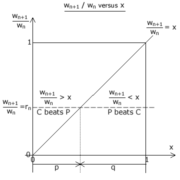
• Hence for C to win, Vw_n+1/xVw_n > 1 and w_n+1/w_n > x

A plot of w_n+1/w_n against x is shown in the figure opposite. The diagonal line represents a tie between C and P as their tallies are equal here. Above this diagonal C beats P and below it P beats C. For a given voting system and pair of adjacent preferences, the ratio r_n = w_n+1/w_n is fixed. The range 0 ≤ x ≤ 1 covers all election profiles.

Hence, the proportion p indicated in the figure above represents the fraction of outcomes where C beats P and the proportion q where P beats C. Note that p + q = 1 and so let the Polarization Index (PI_L) = 1 - CI_L such that CI_L + PI_L = 1.

• Hence, CI_L = p = r_n = w_n+1/w_n
• and PI_L = q = 1 - p = (w_n-w_n+1)/w_n

These two bias indices are illustrated in the figure opposite.

Proceed to next page > Comparisons: Positional Voting 2

Return to previous page > Comparisons: Geometric Voting 11