Comparisons: Condorcet Methods 1

Description of Condorcet Methods

Choosing between just two alternatives is straightforward. The more popular one wins. The Marquis de Condorcet hence developed the idea of reducing multiple-choice decisions to a comprehensive set of two-way (pairwise) ones. Each candidate is compared in turn to every other candidate in a simple pairwise comparison. Should any candidate beat all the others in these pairwise contests, then this candidate is declared the Condorcet Winner of the election. Any voting system that guarantees that the Condorcet Winner (if there is one) always wins the election is regarded as a Condorcet method. As there is often no Condorcet Winner in such methods, each particular method uses a different algorithm to deduce the election winner. For a more detailed and comprehensive description of Condorcet methods, please visit the voting system section of Wikipedia or another reference source.

Properties of Condorcet Methods

Pairwise methods satisfy the majority, summability, monotonicity and Pareto criteria but do not satisfy the consistency and participation ones. As each of the N candidates is compared to each of the N-1 others, this results in N(N-1) or N² - N pairwise comparisons. Therefore, the summability order function is N² (second order) and the count process takes longer than a first order system.

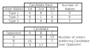
Condorcet methods are clearly a form of preferential voting. The first table opposite defines the input from 24 voters in an example three-candidate Condorcet method election. The second table (called a matrix) presents the results of all the pairwise comparisons. The three winning comparisons are highlighted in white. Here, candidate A beats opponent B as the majority prefer A to B by 16 votes to 8. Similarly, B beats C by 17 votes to 7 and C beats A by 15 votes to 9.

Obviously, there is an inherent paradox here. The three pairwise comparisons produce a 'cyclic' outcome; namely, A beats B, B beats C and C beats A! Not only is there no Condorcet Winner here but there is no clear winner at all. There are many other examples of Condorcet paradoxes when using such methods. The differing variant methods are designed to resolve such intransitive cycles and paradoxes using alternative criteria to determine the eventual winner.

This election example also demonstrates that Condorcet methods fail to satisfy the Independence of Irrelevant Alternatives criterion. If A withdraws, B beats C by 17 votes to 7. If B withdraws, C beats A by 15 votes to 9. If C withdraws, A beats B by 16 votes to 8. Any candidate could win simply depending on which one withdraws. However, some Condorcet methods do satisfy the Independence of Clones criterion while others do not.

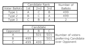
There are 1000 voters in the second three-candidate example election; see table opposite. Polarized candidate A has almost half of all first preferences; as does candidate B. These same type 1 and 2 voters award their lowest preference to the opposing candidate. Only two (type 3) voters cast their first preference in favour of the almost-consensus candidate C. The three winning comparisons are highlighted in white in the pairwise matrix opposite. As C beats both A and B, C is the Condorcet Winner and is ranked first. As B beats A, B is ranked second and A last. There is no cycle or paradox here as the candidate ranking is C then B then A.

This example shows that the essentially consensus candidate C is victorious despite having only two first preferences. Note that this candidate has no third preferences and all but two second preferences.

Like the Borda Count (see Proof CB1), the average rank position of the three candidates can be used instead to determine the candidate rankings; provided no cyclic rankings result from the Condorcet method. The average rank position for candidate C is [(2x1) + (998x2)]/1000 or 1.998th place. Similarly, B is in 2.000th place and A is in 2.002th place. The election ranking is hence again confirmed as C then B then A. Therefore, like the Borda Count, Condorcet methods favour consensus candidates over polarized ones. The winning candidate is the one with the best average performance.

Proceed to next page > Comparisons: Condorcet Methods 2

Return to previous page > Comparisons: Positional Voting 10