Description: Counting

Ranked Ballot

Unlike a number of other preferential voting systems, determining the outcome of a GV/CHPV election is straightforward and transparent. As a positional voting system, it only involves one round of counting as no votes are transferred between candidates. It is only necessary to count the number of each of the preferences separately for each candidate before then multiplying each individual preference tally by its weighting and then summing these weighted preference totals to yield the overall tally for each candidate.

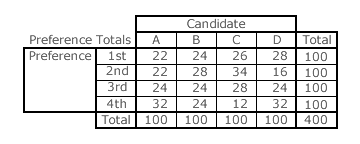
This algorithm can be implemented a number of ways provided full accuracy is always maintained. One recommended approach is to present the preference totals and the weighted preference totals using the tables shown on the right. Notice that in each table, there is one column for each candidate and one row for each preference. In this election example, there are 100 voters and none truncated their preferences. Hence, after counting the number of each of the preferences for each candidate and entering this data into the first table, the row and column totals all then sum to 100; a useful cross-check. Even if some truncation had occurred and not all 400 preferences were cast, this tabular presentation still allows for some cross-checking of voter input.

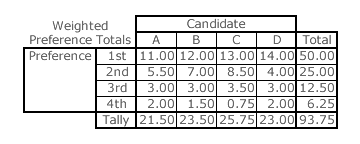
The next stage is to multiply each preference total by its own preference weighting and present these weighted preference totals in the second table (that is identical in format to the first one). In this example, the geometric weightings are one half, one quarter, one eighth and one sixteenth for the four preferences. The row totals can again be used to perform some useful cross-checking. However, it is the column totals that yield the final tally for each candidate on which they will be rank ordered.

Maintaining 100% accuracy throughout is of vital importance. Otherwise, falsely tied rankings or falsely ordered rankings may well occur. In GV, this may restrict many common ratios from being adopted in practice. For example, using one third as the common ratio would be acceptable when kept as an exact fraction (1/3) but not when truncated as a decimal number (0.333....). To avoid fractions altogether, the lowest preference should be weighted as 1 by choosing the appropriate weight for the first preference. Continuing the one-third common ratio example, the weightings for a four-candidate election would then be 27, 9, 3 and 1. The initial weighting has no effect whatsoever on the overall rank-ordering of candidates so any suitable value can be freely chosen in order to simplify the count. Voters should not be confused by being given this irrelevant information. Obviously, election staff and candidates must know all such details in order to determine the outcome and check the accuracy of the result. Voters should however know the common ratio employed as it is critical to the resultant election outcome.

It must be stressed however that GV is not being promoted as a practical voting method but primarily as a very useful analytical tool for evaluating CHPV and comparing it with other competing systems. It is CHPV that is being promoted and accuracy here is very easy to maintain throughout irrespective of the number of voters or candidates. Whether whole numbers, fractions or decimal numbers are used for the weightings, rounding is never necessary nor ever acceptable.

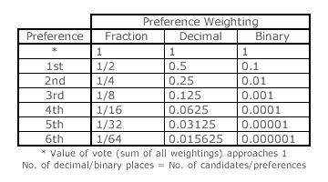
For CHPV, where the common ratio is defined as one half and the initial weighting here is set at one half, the table opposite shows the first six preference weightings expressed as fractions, decimal numbers and even as binary numbers (that electronic calculators and computers use when performing arithmetic operations). These binary numbers clearly show that the CHPV weightings are synonymous with those of the binary number system. CHPV is hence ideally suited to electronic voting. It is obvious by inspecting the table opposite that the number of places needed after the decimal point or binary point is consistently equal to the number of preferences. Therefore, for a finite number of candidates, no rounding or approximation is ever required and none is ever permitted.

Counting in party-list GV/CHPV elections is addressed later in the Description: Party-List section of this chapter.

Proceed to next section > Description: Outcomes

Return to previous page > Description: Voting