Mathematical Proofs: Geometric Voting

Proof CG1: Common Ratio 'Arc' on a Three-Preference Map

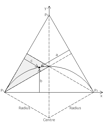
For a three-candidate single-winner election employing a positional voting system, an equilateral triangular map can define and display the three normalised preference weightings used. Such a map is very similar in construction and use to the Three-Party CHPV Maps described in the Map Construction appendix. Here however, each apex represents a weighting of one for the stated preference and the opposing baseline represents a weighting of zero.

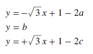
The point shown on the map hence represents a voting system whose weightings are a for the first preference (P₁), b for the second one (P₂) and c for the third (P₃). As for any map, these three co-ordinate values must sum to unity.

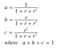
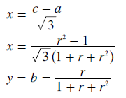
For a GV system, the three preferences must be in the ratio 1:r:r². These weightings can be normalised by dividing each one by the sum of the three. Therefore, the normalised weightings for a GV variant with a common ratio of r are as stated below.

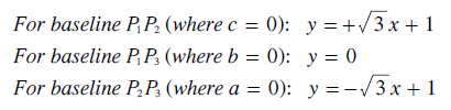
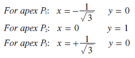
In order to plot each point as r varies, the conventional cartesian co-ordinates (x,y) may be used to replace the weighting co-ordinates (a,b,c). The cartesian origin as at the centre of the P₁P₃ baseline as shown. Bearing in mind that the map is an equilateral triangle with a perpendicular height of one, then the cartesian co-ordinates of the three apexes are as stated below left. The straight line equation for each of the three baselines is also given; below right.

As each weighting varies from zero at its baseline to one at its apex, then the scaling constant k for each weighting can be determined as shown below.

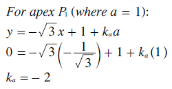
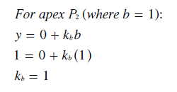
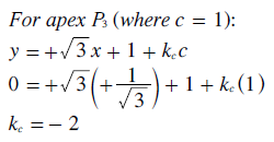
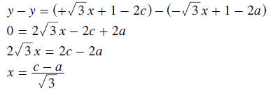
Substituting these three values for k back into their original equations yields the following relationships between the x,y and a,b,c co-ordinates. Clearly, as intended, the y and b co-ordinates are one and the same. By subtracting the first equation for y below from the third one, the transform equation for the x co-ordinate in terms of co-ordinates a and c is easily found as shown below right.

The equations for x and y as functions of a, b and c are now known and those for a, b and c as functions of r are already given above. Hence, using substitution, the equations for x and y as functions of r are given below.

Using these equations, various points representing GV systems with particular common ratios can be plotted on the map. If this is done, it soon appears to be the case that all such points lie on a circular arc where its radius is 2/3 and its centre is offset from the origin at x = 0 and y = -1/3; as shown in the above map. To prove that all points do indeed lie on this arc, the general equation for any circle can be used. For a circle, the square of the radius is equal to the sum of the squares of the x and y co-ordinate values once the appropriate centre offset has been subtracted from each of these values. The equation for this particular circle is hence stated below. The derivation that follows simply shows that the left-hand side of the equation equals the right-hand side thereby proving that all points lie on this circle.

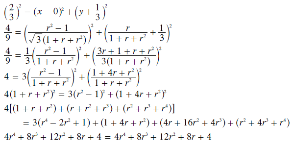
• Therefore, all the points that represent the full range of GV variants from r = 0 to r → 1 form a circular arc from apex P₁ to virtually the map centre.

Notice that the gradient of the arc at the map centre is zero and at apex P₁ it is the same as that of the P₁P₂ baseline.

For a positional voting system to be legitimate, the first preference must be worth more than the last preference and the lower of two adjacent preferences must not have a higher weighting. Otherwise, less-preferred candidates can get promoted over more-preferred ones. Inside the grey region of the map, P₁ has a higher weighting than P₂ and P₂ has a higher weighting than P₃. Hence, any point in another region of the map represents an invalid positional voting system.

Note that the equations used in this proof do not restrict r to be less than one. Here, the common ratio can be anywhere in the range 0 ≤ r ≤ ∞. Hence, the continuation of the arc from the map centre (where r = 1) to apex P₃ (where r = ∞) is also shown on the map. Although values of r above unity are not permitted for legitimate positional voting systems, they remain valid for geometric sequences.

Return to main text > Comparisons: Geometric Voting 1

Refer to > Mathematical Proofs: Table of Contents