Mathematical Proofs: Positional Voting

Proof CV3: Consensus and Polarization Indices for Geometric Voting

The standard positional voting vector for geometric voting with a common ratio of r is given below.

Both bias indices are determined using normalized vectors only. The normalized vector for geometric voting is achieved by subtracting r^N-1 from each weighting and then dividing each one by 1-r^N-1. The resultant normalized vector is shown below.

The formula for calculating each bias index is given in the Consensus and Polarization Indices for Positional Voting Vectors proof. It is however useful to determine the sum of all the preference weightings first. Geometric voting derives its name from the fact that its preference weightings form a geometric progression. As such, the standard mathematical formula for determining the sum of the first N terms in a geometric progression is used here.

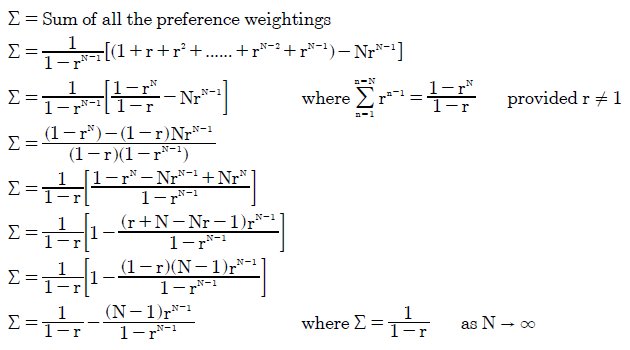
Notice that the sum Σ is a function of both the common ratio r and the number of candidates N. Hence, the two bias indices are also functions of these variables. The first table below shows values of Σ for selected values of r with up to ten candidates. The second table gives the corresponding Consensus Index (CI_V) value for the N-candidate GV(r) vector.

As the number of candidates tends to infinity (N → ∞), the sum Σ simply reduces to 1/(1-r); see above. Therefore, the two bias indices can be greatly simplified here as shown below.

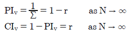
As the number of candidates N increases, the Consensus Index (CI_V) for a GV vector converges towards its asymptote; namely its common ratio value of r.

Return to main text > Comparisons: Positional Voting 5

Refer to > Mathematical Proofs: Table of Contents