
Evaluations: Diagrams and Maps 3
Free, Open and Closed Party Lists
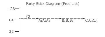
In the preceding election example, party C supporters ranked their three candidates as equals and a tie resulted. If party A and B voters had done the same, then the party stick diagram opposite would display the outcome; a nine-way tie to be resolved by randomly selecting any three from nine. If an extra party C voter had voted, then party C would have won all three seats as each of its candidates would have some additional weighting added to their tally. If instead, one of the party C voters had failed to vote, then party C would not have won any seat as each of its candidates would have some weighting removed.
Hence, a margin of just two votes separates gaining all the seats from gaining none. This extreme example shows just how arbitrary any multiple-winner outcome can be when the ranked ballot CHPV algorithm is used in party-based elections. Using the party-list algorithm instead of the ranked ballot version of CHPV actually produces the identical party stick diagram provided a free list is employed. In both systems, party supporters and not the parties wholly determine the candidate rankings and hence the winners. While limiting the amount of voter input, open lists will still enable some very disproportional results to occur. The only remaining option is for the party-list CHPV algorithm to use a closed list instead.
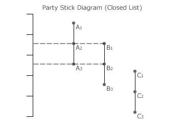
In the three-party three-winner closed party-list example opposite, party A has twice the support of party B and both have much greater support than party C. Candidates A2 and B1 are necessarily but non-critically tied. Together with A1, they are elected to fill the three seats. Hence, party A has two seats while party B has one. This is an exactly proportional ratio between tally share and seat share for these two parties. As party C has some support but no seat, the election outcome is optimal but not truly proportional.
By using the closed party-list approach, this CHPV algorithm is potentially capable to producing reasonably proportional multiple-winner outcomes. This potential is evaluated in great depth in the remaining sections of this chapter. However, once party seat shares have been determined using the closed party-list algorithm, then the ranked ballot algorithm can still be used by party supporters for the selection of candidates to fill the seats won by their party.
Party stick diagrams (especially when computer animated) are effective in displaying how voter input changes affect CHPV election outcomes. However, they are particularly useful evaluation tools when formally assessing the party proportionality of multiple-party multiple-winner CHPV elections. They are used extensively with maps to analyse critically tied situations and hence to determine the boundaries between different election outcomes (share of seats) on such multiple-party multiple-winner CHPV maps.
Two-Party Maps
The relative share of the vote for one party is simply its own tally divided by the sum of all such party tallies. By definition, these tally shares (t) must total to unity. Hence, by determining the tally shares for all but one party, then this particular party must have the remaining share. So, if the number of candidate sets (parties) is S, then the number of variable tally shares to be handled is S - 1. When mapping them, one dimension less than the number of parties is hence required.
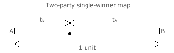
Therefore, the two-party single-winner map opposite only needs the one axis. Party A has its tA share and so party B has the remainder (tB = 1 - tA). Notice that the distance from the opposite end towards end A represents tA and the remainder towards end B represents tB. With only two parties and one candidate each for the single seat, whichever candidate gets the larger tally share is ranked first and the other second.
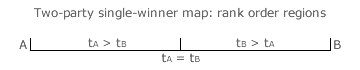
When both receive the same share (half each), they are then critically tied and one must be selected at random as the winner. This critical tie (where tA = tB) is shown on the map opposite. The left-hand half of the map is the region where the rank order is A then B (as tA > tB) and the right-hand half is the region where the rank order is B then A (as tB > tA).
Proceed to next page > Evaluations: Diagrams & Maps 4
Return to previous page > Evaluations: Diagrams & Maps 2