Evaluations: Optimality of CHPV 2

Mismatches between CHPV and OPV Domain Boundaries and their Consequences

By definition, an OPV system will minimise the discrepancies between tally shares and seat shares for the parties overall. Hence, to gain a first or subsequent seat, a party must exceed the relevant proportional tally share threshold. Such thresholds correspond to the domain boundaries on a OPV map. As the boundaries for CHPV are displaced with respect to OPV ones, a party may gain a particular seat with a lower or higher tally share in a CHPV election compared to a OPV one.

Consider the case of two parties (S = 2) competing in a party-list election with W winners. With OPV, each of the W seats equates to a proportional tally share of 1/W. For a party to win its first seat it must exceed half of this share (t > 1/2W) as optimum proportionality requires rounding to the nearest whole share. With CHPV, does a party need the same share to win its first seat? Or a higher or lower share? If the threshold is raised with CHPV, then some bias against the smaller party exists. If it is lowered, then some bias occurs in its favour instead. So, the magnitude and sign of the difference in the corresponding pair of CHPV and OPV tally share thresholds respectively reflect the extent and direction of any inherent bias regarding the size of party support in the party-list CHPV election.

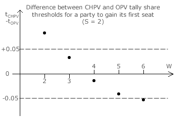
Initially, suppose there are two seats (W = 2) in this election. For a party to win its first seat in an OPV election, it must exceed a tally share of 1/2W or 1/4 here. Under CHPV, it must achieve more than half that of the other party; namely over 1/3 compared to under 2/3 for the larger party. The difference between the CHPV and OPV tally shares is hence 1/3 minus 1/4 or +1/12. This difference is plotted on the graph opposite.

The tally share difference for elections with three, four, five and six winners is similarly calculated and these differences are also shown on this graph.

The relevant CHPV and OPV tally share thresholds for a party to gain its first seat are clearly displayed in the various two-party multiple-winner maps on the CHPV Maps 1 page. They correspond to the domain boundaries closest to the left-hand end of a map (for party A). Both the sign and the magnitude of the difference between any corresponding pair of thresholds are fully visible.

From the graph, it is clear that CHPV is not inherently biased for or against a small party. Any bias depends on the number of seats to be filled. For two or three winners, there is a slight disadvantage for the smaller party. For four or more, the smaller party has a slight advantage instead. If a smooth curve is drawn through the dots on the graph, it would intercept the zero tally share difference axis at about W = 3.7. It is at this point that optimality is at a maximum.

With less than this value (two or three winners), the bias is against the smaller party and this bias grows as W decreases. With more than this value (four or more winners), the increasing bias is now in favour of the smaller party. The two-party bar chart on the previous page also reflects this peak in optimality at around W = 3.7 too as it steadily declines either side of this peak. For two parties, the number of seats needed for maximum optimality is either three or four. Where any marginal systemic bias against the smaller party is desired, the lower number should be chosen.

As the number of winners becomes large, the smallest tally share threshold to gain a seat becomes unacceptably low and disproportionate. Hence, the number of seats in a reasonably proportional CHPV election is limited by the degree to which the bias towards a small party is acceptable. Hence, party-list CHPV is necessarily restricted to few-winner elections.

For a CHPV election with three parties (S = 3) and W winners, the required tally share threshold for a small party to gain its first seat varies somewhat according to how the other two share the remaining tallies between them. By inspecting the three-party multiple-winner maps on the CHPV Maps 2 and CHPV Maps 3 pages, the differences between the CHPV and OPV domain boundaries for critical ties between no seats and one seat for a party can be observed. For up to four winners, the majority of the thresholds are raised indicating some bias against the smallest party. For six or more winners, the majority of them are lowered so there is now some bias towards the smallest party.

The peak in optimality appears to be around five winners as roughly as many thresholds are raised as are lowered. Below this peak (W < 5) there is a marginal bias against the smallest party and above it (W > 5) this bias reverses in favour of the party. The magnitude of any bias grows as the number of winners steadily diverges from this optimum of five.

Therefore, there is negligible bias towards or against the smallest party gaining its first seat when there are about five seats to be filled. However, with three parties, optimality reaches its peak with four winners; see the three-party bar chart on the previous page. The contrast is in fact due to the tally share threshold for a party to gain its second seat. The CHPV and OPV domain boundaries (for critical ties between winning two seats or one) are closer with four winners than with five.

Hence, with four seats, there is a probability of a slight bias against a party winning its first seat but one towards it when seeking its second seat. Given the varying size and shape of CHPV domains on a map, such distortions whether large or small are clearly inherent. To minimise any bias in a CHPV election, it is best to employ the number of seats that yields maximum optimality or to round this number down to prevent any small party from gaining a seat too easily.

Proceed to next page > Evaluations: Optimality 3

Return to previous page > Evaluations: Optimality 1