Evaluations: Optimality of CHPV 4

Proportion of Optimal Outcomes in Multiple-Party Multiple-Winner CHPV Elections (continued)

Ideally, for perfect optimality, the extreme seat share domains for CHPV would be synonymous in both shape and size with those for OPV and therefore yield a CHPV/OPV ratio of one. Although the domain shapes can never be equal, the approximation model requires that their sizes should be as equal as possible. So the closer this ratio is to unity, then the better CHPV performs in terms of optimality.

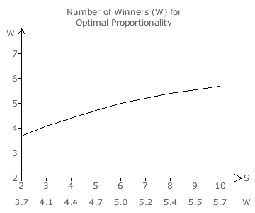
For a given number of parties (S), the optimum number of winners (W) can be determined by equating the relevant CHPV/OPV ratio (see previous table) to unity and solving for W. Although the number of winners or seats is an integer, the values of W obtained by this method are not. These values of W for between two and ten parties are calculated to one decimal place and are shown underneath the graph opposite.

The graph itself shows a continuous curve through all of these values. This graph is only intended to show the relationship between the number of seats and the number of parties. The value of W for any given S should always be rounded to the appropriate integer.

As the number of parties contesting an election increases, the number of seats needed for maximum optimality also increases but its growth steadily declines. Using the extreme seat share domain approximation model, then about four or five winners is the optimum number for up to nine parties.

At least for two-party and three-party CHPV elections, these approximate results for maximum optimality can be compared directly to the actual precise ones.

For two parties, the CHPV and OPV extreme seat share domains are at their closest in length when there are four winners; see the CHPV Maps 1 page. The approximate value (W = 3.7) agrees with this actual one (W = 4) when rounded to the nearest integer. For three parties, the domains are closest in area when there are also four winners; see the CHPV Maps 3 page. The approximate value here (W = 4.1) again agrees with the actual one (W = 4) when rounded to the nearest integer. The approximation model is hence a reasonable basis on which to extrapolate the optimum number of seats to be awarded for an anticipated number of parties competing in a party-list CHPV election.

For three parties, the preceding bar chart shows that maximum optimality occurs with four winners. This is also the condition for the CHPV and OPV extreme seat share domains being closest in area. For two parties, this bar chart shows that maximum optimality occurs with three winners. However, the two extreme seat share domains are at their closest in length with four winners and this same situation ensured minimal bias in favour of the smaller party. Although rounding W to the nearest integer is appropriate for domain volume ratio equality, it is better to round W down to the nearest integer for deducing the number of winners that is needed for maximum optimality. Here, any lack of optimality then favours larger parties.

On this basis, maximum optimality is achieved in party-list CHPV elections with four seats where three to five parties compete or with five seats where six to ten parties compete. As any outcome in such a multiple-party multiple-winner CHPV election is highly party proportional, there are likely to be more parties nominated than seats available. Therefore, without knowing the number of parties that will stand, optimality within CHPV is likely to be maximised with five seats.

A significantly large number of parties (S > 10) might enter such a few-winner CHPV election. However, the number of seats needed to maintain optimality is unlikely ever to exceed six in practice. A contest with a very large number of winners simply introduces too much distortion in favour of small parties and so results in highly disproportional outcomes. Therefore, a 'few-winner' multiple-party CHPV election is defined as one where no more than six seats (W ≤ 6) are to be won and where W is typically four (for S ≤ 5) or five (for S ≥ 6) to achieve maximum optimality.

For party-list CHPV, any bias towards or against small parties can be controlled by choosing the number of seats for a given election. Where a minimum threshold is required as a barrier against too small a party getting a seat, then the number of winners should be marginally lower than its optimal value. There is clearly a trade-off here between introducing such a barrier and maintaining optimum proportionality. It is important to reiterate that maximum optimality and minimal systemic bias to any party are 'two different sides of the same coin'. So there is inherent harmony here regardless of the number of parties or winners.

Proceed to next section > Evaluations: Party Cloning

Return to previous page > Evaluations: Optimality 3