Evaluations: Optimality of CHPV 3

Proportion of Optimal Outcomes in Multiple-Party Multiple-Winner CHPV Elections

For five or more parties, it is not possible to map every election outcome as more than three dimensions would be required. For four parties, a three-dimensional map can be produced but it is difficult to view or interpret such a solid object.

Looking back again at the earlier three-party maps, it is noticeable that when CHPV domain boundaries are closest to matching OPV ones (namely W = 4 for maximum optimality), the three corner domains for CHPV and for OPV are also at their most similar. Likewise, for the two-party maps, when the CHPV seat share thresholds are closest to matching the OPV ones (namely W = 3 for maximum optimality), the two end domains for CHPV and for OPV are almost at their most similar too. Only for four winners (W = 4) are they very slightly closer.

Hence, as an approximation, these 'extreme' seat share domains can substitute for the maps as a whole in terms of identifying the number of winners needed for maximum optimality. The term extreme refers to any domain where all the seats are won by one party and none by the others. The term 'volume ratio' is used below for the 'size' of a multi-dimensional domain relative to the 'size' of its host multi-dimensional map. The volume ratio for each such extreme domain as a function of the number of seats/winners (W) in two-, three- and four-party elections are listed in the table below for both OPV and CHPV.

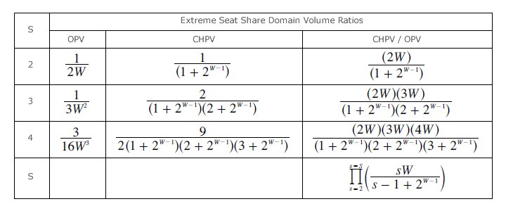
[Note: For the two-, three- and four-party maps and their extreme seat share domains, please refer to the proofs opposite.]

To compare the optimality of CHPV against the 100% benchmark of OPV, another ratio can again be employed; see the end column in the above table. If their respective volume ratios are similar in value, then the ratio of these two volume ratios should be close to unity. The CHPV/OPV ratios shown here have deliberately been left unsimplified so that the pattern that emerges as each additional party is included is obvious. Given this clear progression, the comparative CHPV/OPV ratio for two-, three- and four-parties can easily be extended to further parties. [Note: The mathematical formula for this ratio as a function of the number of competing parties (S) is given in the final cell.]

Proceed to next page > Evaluations: Optimality 4

Return to previous page > Evaluations: Optimality 2