Mathematical Proofs: Geometric Voting

Proof CG6: Rank of the Preference with the Mean Weighting

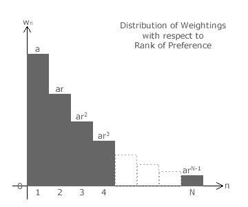
In GV, the weighting (w_n) of each preference is defined by its rank position (n). The bar chart opposite shows the distribution of these weightings with respect to the rank of the preferences for an election with N candidates.

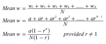
The mean weighting is then simply the sum of all these weightings divided by the number of them; see below. The following calculation then uses the standard equation for the sum of the first N terms of a geometric sequence to simplify the expression for this mean weighting.

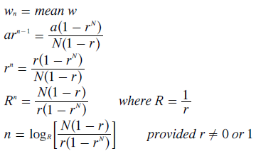
Let the preference with the mean weighting be P_n where its rank position is n. Hence, this preference has a weighting of w_n as well as the mean w. By equating and simplifying this relationship, the rank position n can be found for any given r and N; as shown below.

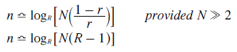
For a large number of candidates standing in an election, this rank position equation can be simplified further. The approximate relationship with the number of candidates greatly in excess of the minimum number required is given below.

For CHPV (GV with r = 1/2), this approximation reduces further to a very simple one as stated below.

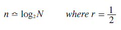
This is a well-known equation in information theory. It defines the number (n) of 'binary digits' or bits needed to encode N different 'things' where binary logarithms (log₂) are naturally used for binary digits. Here however, the equation identifies the rank position (n) of the preference (P_n) with the mean weighting when using CHPV.

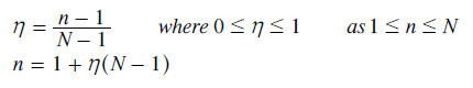
The rank position (n) for the first preference (P₁) is one and for the last preference (P_N) is N. In order to compare the rank position of the mean-weighted preference with those of the highest- and median-weighted ones, it is convenient to use a per-unit measure of rank position (η). This per-unit rank η is defined below where η is zero for P₁ and one for P_N.

In GV, the highest-weighted preference is always the first preference P₁ so η is always zero irrespective of r or N. As the weightings in GV are already in rank order, the median-weighted preference is simply the middle one. Hence, η is always 1/2 here; again irrespective of r or N.

However, the mean-weighted preference does vary with r and N. The above equation relating the nth weighting to the mean weighting is reworked below to yield the equation for η as a function of r and N.

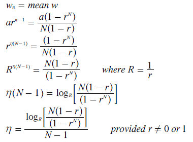
For a set of selected common ratios (r), graphs of η against N can now be plotted (see main text) to show how the rank of the preference with the mean weighting varies with r and N and also with respect to the invariant highest-weighted preference (where η = 0) and median-weighted preference (where η = 0.5).

Return to main text > Comparisons: Geometric Voting 6

Refer to > Mathematical Proofs: Table of Contents