Comparisons: Geometric Voting 6

Preference Weightings and Rankings for Consensus

It is already clear that the Borda Count favours more consensual candidates with broad yet relatively weak support over more polarized ones with strong but narrow support. The reverse is true for plurality (FPTP) elections. How does the GV common ratio affect the balance between these two extremes? One means of assessing this spectrum is to determine the minimum winning rank of a preference awarded unanimously to a candidate. Assuming no truncation, this rank is achieved when all the other candidates are tied with the same tally. If they were not tied, then the top-ranked candidate would have a higher tally for the consensus candidate to overcome. The following two statements apply to this scenario.

• The minimum winning rank of the preference awarded to the consensus candidate is always greater than the rank of the preference with the mean weighting.

• A candidate with a unanimous preference from every voter can never win when the rank of this preference is lower than the mean-weighted one.

Preferences with a weighting above the mean value are hence defined as being of high rank and, conversely, those with a weighting below the mean value are of low rank. In trying to establish a winning candidate tally, high preferences are essential while low preferences are a hindrance.

The mean weighting awarded by a voter is the sum of all the preference weightings (from w₁ to w_N) divided by the number of preferences (N). Therefore, the average candidate tally contribution awarded by a voter is equal to this mean weighting. So how does the rank of the preference with the mean weighting vary according to both the number of candidates (N) and the weightings as determined by the common ratio (r)?

• Employing CHPV (GV with r = 1/2), the rank position (n) of the mean-weighted preference is approximately equal to the binary logarithm of the number of candidates (n ≅ log₂N).

For example, the mean-weighted preference in an eight-candidate election is the third preference; as log₂(8) = log₂(2x2x2) = log₂(2³) = 3. Similarly, with four or sixteen candidates, the mean-weighted preference is the second or fourth one respectively; since log₂4 = 2 and log₂16 = 4. With say ten candidates, the mean-weighted preference is between the third and fourth ones; as log₂10 = 3.322. No such individual preference exists as rank position is clearly an integer. To stand any chance of winning, a consensus candidate must nevertheless receive a preference that is ranked higher than 3.322th place. So, a fourth or lower preference guarantees defeat.

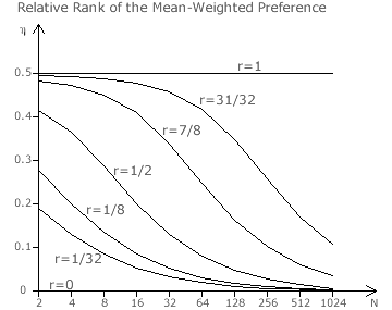
For GV in general, it is useful to use a per-unit indicator (η) of rank position rather than n. Therefore, for the first preference (P₁) η is 0, for the last preference (P_N) η is 1 and for the middle preference η is 1/2. For GV with r → 1 (or the Borda Count), this middle preference (where η = 0.5) has the weighting equal to the mean; as the weightings sequence is linear. For GV with r = 0 (or FPTP), only the first preferences (where η = 0) matter. The relative (per-unit) rank of the mean-weighted preference in other GV systems is stated below (where R = 1/r).

• η = log_R[N(1-r)/(1-r^N)] / (N-1)

The graph opposite shows the variation in relative rank (η) as a function of the number of candidates (N) for each of the stated values of the common ratio (r). It is important to notice two key features of the GV graph.

• The mean-weighted preference P_n is always between the first and middle preferences (0 ≤ η ≤ 0.5).
• The relative rank of P_n rises (lower η) as r becomes smaller or as N becomes larger.

Not only is η an indicator of the relative rank of the mean-weighted preference but it is also a good indicator of the extent to which the chosen GV system promotes consensus candidates. FPTP and GV with low values of r do not favour consensus candidates but the Borda Count and GV with high values of r do promote them. As η declines, it becomes progressively more difficult for a consensus candidate to beat a polarized one.

For example, consider a GV election where the mean-weighted preference has a relative rank of 1/4 (η = 0.25). To stand any chance of winning, a consensus candidate must therefore receive a unanimous preference from the top quartile of rank positions from every voter. One from any of the other three quartiles ensures defeat.

In reality, candidates are rarely perfect consensus or polarized ones but somewhere in-between. Nevertheless, a candidate must receive a sufficiently large number of sufficiently high-ranked preferences to win. As η varies with the common ratio, the balance between the quality (rank) and quantity of these preferences needed for victory changes.

Proceed to next page > Comparisons: Geometric Voting 7

Return to previous page > Comparisons: Geometric Voting 5