Comparisons: Positional Voting 8

Bias Indices for A-GV(r) and C-GV(r)

As explained on page 3 of this chapter, every vector has its corresponding A-GV(r) and C-GV(r) ones. GV(r) vectors range from GV(r=0) to GV(r→1) only since the sum of all the normalized weightings of such a vector must not exceed half the total number of weightings so 1 ≤ Σ ≤ N/2. Conjugate vectors occupy the remaining range where N/2 ≤ Σ ≤ N-1. However, recall that C-GV(r) and A-GV(r) are equivalent for the same r and hence have the same system bias.

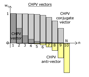
The relationships between a vector, its anti-vector and its conjugate vector are illustrated opposite for N = 10 using CHPV as an example of a GV(r) vector. Notice that the sum Σ is less than N/2 for the (dark grey) vector but greater than N/2 for its (dark plus light grey) conjugate vector. As always, these two sums total to N. In contrast, the sum Σ for a vector and its (yellow) anti-vector are always equal in magnitude.

The figure below opposite illustrates how the bias indices vary as the common ratio r is increased in steps of 1/4 from 0 towards 1 for a GV(r) vector and then from here back to 0 for a C-GV(r) or A-GV(r) one. This example employs ten candidates.

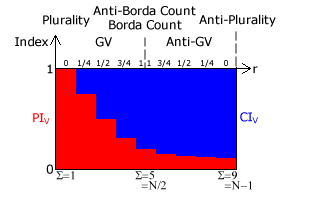
For Plurality and GV(r=0), this vector is wholly polarized as Σ = 1. For the GV(r=1/2) or CHPV vector, it is essentially balanced as Σ = 1.98 and the two bias indices are almost equal in value. For the Borda Count or GV(r→1) vector and the Anti-Borda Count or A-GV(r→1) anti-vector, Σ = 5 = N/2 and PI_V = 1/5 = 0.2. Across the range of vectors, Plurality is the most polarized and the Borda Count is the most consensual.

However, across the range of anti-vectors, the Anti-Borda Count is the least consenual and Anti-Plurality the most as Σ = 9 = N-1 and CI_V = 0.888. Note that any anti-vector is more consensual than any vector. Also note that there is no discontinuity in the transition from vectors into anti-vectors as the Borda Count vector and Anti-Borda Count anti-vector are identical.

Teaming Thresholds for A-GV(r) and C-GV(r)

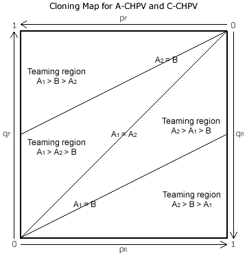
Cloning maps for GV(r) vectors are introduced in the earlier Evaluations: Teaming Thresholds chapter. They can also be constructed for A-GV(r) and C-GV(r). As an example, a cloning map for A-CHPV and C-CHPV is shown opposite. Here, candidate B is competing against clone candidates A₁ and A₂ but had there been only one A candidate then A and B would have tied for first place.

Above the A₁ = B tally threshold, A₁ beats B through teaming. Similarly, below the A₂ = B one, A₂ beats B through teaming. As these two teaming regions therefore overlap between the two thresholds, there is no vote-splitting region on this map. Within a teaming region, B is pushed into second place but, where two of them overlap, B is pushed further down into third place. Only at the top (or bottom) of the map does B tie with A₁ (or A₂) in first place. Nowhere within the map does B ever win.

For any A-GV(r) anti-vector or C-GV(r) conjugate vector, the two teaming regions always overlap. The closer it is to Anti-Plurality, the larger each region becomes and the bigger the overlap. There is never any vote-splitting region on the map for an anti-vector. Therefore, all A-GV(r) anti-vectors are inherently vulnerable to teaming to the extent that it all but guarantees victory to a clone candidate. Further, there is no defence against such strategic nominations except for B to clone itself too. Potentially, ‘runaway’ cloning may then spiral out of control.

Proceed to next page > Comparisons: Positional Voting 9

Return to previous page > Comparisons: Positional Voting 7