Comparisons: Geometric Voting 3

Effect of Exchanging Preferences between Candidates

During an election campaign, candidates will seek to maximise the value of preferences awarded to them and to minimise those given to their competitors. When using geometric voting or indeed any other a positional voting system, this means trying to persuade voters to grant them a higher rank to the detriment of others. This exchange of preferences by the re-ordering of candidates on the ranked ballots may have a significant or negligible effect on the candidate tallies. For GV, it depends very much on the value of the common ratio that is employed.

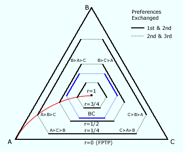
A standard three-party single-winner CHPV map is shown opposite; see the Three-Party CHPV Maps section again for more details. Here, there is only one candidate per party so A, B and C represent the three candidates (rather than parties) in this contest. It is important to recall that the proportional distance from the opposing baseline towards an apex represents the per-unit value of the preference awarded to that particular candidate. For example, if a voter in a CHPV election ranks the candidates as A first and C last (A>B>C), this is represented on the map as a point that is 4/7 towards apex A, 2/7 towards apex B and 1/7 towards apex C.

If the voter decided to swap their preferences for first and second place (B>A>C), then a new point is created on the map. The relevant solid line on the map connects these two points and highlights the significant effect of this exchange. If the voter had instead just switched their preferences for second and third place (A>C>B), then the relevant dotted line on the map illustrates the smaller effect of this other exchange. By considering all the six possible sequential exchanges of adjacent preferences, the irregular hexagon for GV with r = 1/2 (CHPV) is formed.

For the Borda Count (BC), a similar hexagon can be constructed. Notice that it is a regular hexagon as any exchange of adjacent preferences has the same per-unit value since there is a common difference of 1/6 between the three weightings of 3/6, 2/6 and 1/6. For GV with r tending to 1, its weightings approximate to 1/3, 1/3 and 1/3 with a common infinitesimally small difference between adjacent weightings. Therefore, exchanging any preferences is of no consequence and the point in the centre of the map represents its miniscule hexagon.

For first-past-the-post (FPTP) or GV with r = 0, another hexagon can be formed. However, exchanging preferences for second and third places has no effect as each has zero value. Hence the three dotted lines of this hexagon have zero length so leaving the three solid lines to form an equilateral triangle. This triangle equates to the periphery of the map since exchanging first and second preferences generates the maximum possible shift in value; namely 1.

For comparison, two further hexagons are shown on the map. One is for GV with r = 1/4 and the other is for GV with r = 3/4. The red arc from apex A to the map centre that is shown on the previous page is repeated on the map here too. This arc connects all the points that represent the ranking A>B>C in GV regardless of the common ratio used. Similar arcs may be drawn for the other five rankings. [The GV hexagons are those shown in black while the non-GV Borda Count one is shown in blue and should be ignored when considering the effect of varying the common ratio.] As the value of r increases from zero and steadily progresses towards one, the hexagon becomes less irregular in that the ratio of the three shorter sides of the GV hexagon to the three longer ones also evolves from zero to almost one. Indeed, both are the common ratio by definition. As they vary with r, the hexagons on the map provide a good visual interpretation of the effect of exchanging preferences within GV.

Proceed to next page > Comparisons: Geometric Voting 4

Return to previous page > Comparisons: Geometric Voting 2