
Comparisons: Geometric Voting 5
Three-Candidate Elections and Maps (continued)
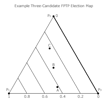
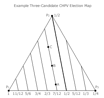
A three-candidate map complete with the primary iso-tally grid line (shown in bold) and any desired secondary ones can now be displayed. Where the chosen method is the FPTP voting system (or GV with r = 0), its map is shown opposite. For the CHPV system (GV with r = 1/2) and the Borda Count one (or GV with r→ 1), the maps are given below.
Recall that the preference shares are fixed so each candidate dot is in the same position on each map. It is important to remember that the voter input determines the position of each dot and it is the voting system (value of r) that determines the placement of the iso-tally lines.
The collective ranking of the candidates can now be determined visually using the grid lines. The average tally per voter (t) associated with successive iso-tally lines is in ascending order from apex P3 towards apex P1. Only displacements at right-angles to the grid lines should be considered when determining the candidate rankings.
For the FPTP election, candidate A has a tally just higher than 0.4 and B has one nearer to 0.4 than to 0.2. Candidate C has a tally nearer the 0.2 grid line. It is immediately clear from the map that A is ranked first with B second and C last. This is confirmed by the actual t values of 0.417, 0.333 and 0.25 (given the P1 shares of 5/12, 1/3 and 1/4).
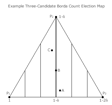
For the Borda Count election, candidate C has a tally higher than the second preference (r = 1 - δ) while A has a tally lower than it and B is in-between. Despite δ tending to zero and all t values tending to one, the outcome rank order is clearly C then B then A. The voting system shown here is really GV with r → 1. However, as demonstrated earlier, it always produces the same candidate rankings as any other Borda Count election irrespective of the value of the common difference.
For the CHPV election, all three candidates have a tally that lies on the 7/12 grid line. There is therefore a three-way tie for first place. Hence, in this illustrative election, any common ratio in the range 0 ≤ r < 1/2 will produce the rank order ABC while one in the range 1/2 < r < 1 will produce the completely reversed CBA ranking.
Using three-candidate maps, it is literally very easy to see how outcomes vary according to which positional voting system (which r) is chosen for any given three-candidate election profile (any voter input).
Proceed to next page > Comparisons: Geometric Voting 6
Return to previous page > Comparisons: Geometric Voting 4