Comparisons: Geometric Voting 7

Balancing Polarization and Consensus

For a given GV election, the common ratio to be employed and the number of nominated candidates is fixed and both are known during the campaign for voter support. From the preceding page, a low preference is by definition one that makes a below-mean-weighted contribution to any candidate tally. Relative to an average contribution, this only worsens the chances of victory for the particular candidate. Attracting only low preferences guarantees defeat.

A potentially winning candidate must attract a large proportion of the above-mean-weighted (high) preferences to achieve success. Over the course of the campaign, it is obviously beneficial to improve both aspects. But which is the more important, the quality (rank) of the high preferences or the quantity of them?

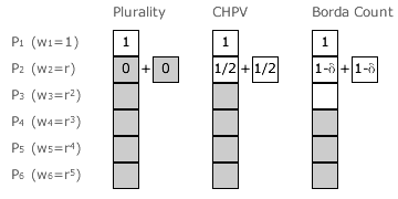
The preference figure opposite relates to a GV election with six candidates (N = 6) and three different values of the common ratio. For GV with r = 0, the outcome is equivalent to plurality (FPTP) and, for GV with r = 1 - δ where δ → 0, it is equivalent to the Borda Count. These two extreme positional variants are also compared to the central CHPV one where r = 1/2.

Let P_H and P_L respectively be the higher and lower preferences of two that are adjacent in rank. Hence, if P_H has a weighting set at one, then P_L is weighted at r. Is it better for a candidate to be awarded one P_H preference or two P_L ones? To put the same question another way round, is it better to try to convert a P_L preference into a P_H one or to attempt instead to obtain a second P_L one?

First consider the campaign strategy for the GV (with r = 0) and plurality (FPTP) scenarios. The mean weight of the six preferences is simply 1/6. So the rank position of this mean-weighted preference is somewhere between the first and second preferences as w₁ = 1 and w₂ = 0. There are hence five low preferences but only the first preference is a high one. In the above figure, high preferences are shown as white cells and the low ones as grey cells. Candidates in these elections must therefore concentrate on maximising the quality of their preferences as only the highest rank counts.

Next, consider the situation for the Borda Count. The mean-weighted preference has the middle rank position of 3.5th place. Therefore, the first, second and third preferences are the high ones while the fourth, fifth and sixth ones are low preferences. For any pair of adjacent high preferences, P_H is only worth δ more than P_L where δ tends to zero. So two P_L preferences are worth virtually double one P_H preference. Clearly, Borda Count candidates should not worry unduly about the rank of their high preferences but should focus instead on maximising the quantity of them.

Finally, consider the CHPV scenario. The rank of the mean-weighted preference is about 2.6th place (as log₂6 ≅ 2.6); see the previous page. For this CHPV election, there are therefore two high preferences and four low ones. With r = 1/2, two P_L preferences and one P_H preference are worth exactly the same. Converting a P_L preference into a P_H one contributes an identical amount to a candidate tally as having an additional P_L preference instead. Therefore, the campaign strategy for a CHPV candidate is to maximise both the quality and quantity of their high preferences as both count equally.

It is again clear why plurality favours polarized candidates over consensus ones and why the Borda Count favours the reverse. For FPTP, candidates must focus exclusively on getting top-rank support. For the Borda Count, they must focus instead on increasing the proportions of their high preferences. As the need for quality versus quantity is evenly balanced, CHPV is hence the optimum consensual GV variant mid-way between the polar extremes of plurality and the Borda Count. It is not biased in favour of either polarized or consensus candidates.

Proceed to next page > Comparisons: Geometric Voting 8

Return to previous page > Comparisons: Geometric Voting 6