Comparisons: Geometric Voting 4

Three-Candidate Elections and Maps

As any three-candidate positional voting election is equivalent to GV with the appropriate common ratio, an example election can illustrate how the collective candidate rankings vary considerably according to which system is employed. In other words, how such rankings depend on the value of r. For comparison purposes, the voter input to this election is fixed and is detailed opposite.

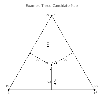
The share of first, second and third preferences for each candidate is however better presented on a three-candidate map; see opposite below. Such a map is very similar in construction and use to the Three-Party CHPV Maps described in the Map Construction appendix. Here however, each apex of the equilateral triangular map represents a full share for the stated preference and no share for the other two. For example, apex P₁ represents a candidate with a first preference from every voter.

The share (v₁) of first preferences (P₁) obtained by candidate B is 8 from 24 so v₁ equals one third. Similarly, B has a one-third share (v₂) of second preferences (P₂) and also a one-third share (v₃) of third preferences (P₃). The dot in the centre of the map therefore represents the three per-unit preference shares for candidate B. Each share is positioned in the direction of the relevant apex (where v = 1) at right-angles to its opposing baseline (where v = 0); as shown on the map. The three share values necessarily sum to one; the key property of any such map. The position of the dots for candidates A and C are similarly determined and plotted.

It is important to note that the position of each candidate dot on the map is fixed irrespective of the common ratio chosen as it simply records their share of the preferences awarded by the voters. What does vary with the common ratio is the candidate tally that results from the weightings of these preferences.

For convenience, the GV weighting of a first preference is set to 1 with r and r² then being the second and third preference weightings. Rather than determining the absolute tally (T) for candidates, the average tally per voter (t) is more convenient. The rank ordering of the candidates is the same whether T or t is used. All voters award the same relevant preference at apexes P₁, P₂ and P₃. As the average tally per voter at an apex is equal to the weighting of the one and only preference expressed here, these apexes represent t values of 1, r and r² respectively.

In order to see the collective candidate rankings directly on the map, iso-tally grid lines need to be superimposed onto the map. An iso-tally line is one where every point along it has the same average tally per voter associated with it. The position and orientation of these grid lines naturally vary according to the common ratio (r). It is this variation that ultimately reflects the differences in the rankings. The primary iso-tally line is defined as the one where the average tally per voter (t) is equal to the weighting of a second preference (r). Iso-tally grid lines are defined as follows.

• The primary iso-tally grid line (where t = r) is a straight line between apex P₂ and the point on the linear P₁P₃ baseline whose value is r.
• Any secondary iso-tally grid line for tally t is parallel to the primary one and intercepts the linear P₁P₃ baseline at the point whose value is t.

On the next page, primary and secondary iso-tally grid lines are displayed for maps that are specific to the chosen GV common ratio.

Proceed to next page > Comparisons: Geometric Voting 5

Return to previous page > Comparisons: Geometric Voting 3