Comparisons: Geometric Voting 8

Balancing Vote Splitting and Teaming

Plurality suffers from vote splitting but not teaming. The Borda Count suffers from teaming but not vote splitting. GV variants between these extremes exhibit both features but with one increasing in magnitude as the other declines. There is in fact only one value of the common ratio that achieves an equal balance between these two magnitudes; r = 1/2.

• CHPV is the only GV variant that achieves an equal balance between vote splitting and teaming.
  Refer to proof CG7

The cloning map with the four pairs of CHPV teaming thresholds presented on the Evaluations: Teaming Thresholds 4 page is repeated below left. Plotted on this map is a red path and four dots. The graph below right records the tally ratio (T_A/T_B) for each of the two clones A₁ and A₂ along this red path from dot 1 to dot 4. The equations for the two tally ratios are also derived in proof CG7. The specific values plotted on the graph are calculated using these equations.

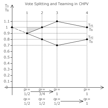
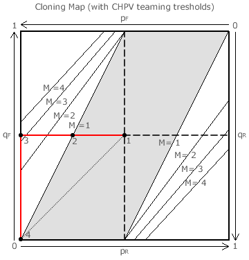
Prior to cloning, there is a critical tie between the two candidates A and B. This presents the easiest opportunity for A to win through teaming by replacing its candidate with its two clones. Dot 1 represents the situation where the two identical clones have been substituted for A. Here, p_F = q_R = 1/2 as the forward slate has yet to be issued. The two identical clones necessarily have the same tally ratio of 0.9 and, under CHPV, this results in vote splitting with a magnitude of 0.1. In other words, each A clone has lost 10% in comparison with the pre-cloning tally for A.

Dot 3 represents the situation after the A supporters vote according to their forward slate but before the B supporters respond to this teaming attempt. Here, p_F has increased to 1 while q_R remains at 1/2. The tally ratio for the superior fraternal clone (A₁) has now increased to 1.1. Hence, under CHPV, A has successfully teamed against B by a factor of 10%. Notice that this factor has the same magnitude as that for vote splitting.

On both the map and the graph, the grey areas correspond to cases of vote splitting and the white areas to cases of teaming; since M = 1 here. Dot 2 is mid-way between dots 1 and 3. This is where only half of A supporters adhere to the slate. Between dots 1 and 2, vote splitting occurs and, between dots 2 and 3, teaming occurs. As for dots 1 and 3, consider any two points on the red path on opposing sides of dot 2 but equidistant from it. Ignoring the sign but not the magnitude, these two points exhibit the same difference between the actual tally ratio and the one for the critical tie (tally ratio = 1). Dot 4 represents the restoration of the critical tie when B supporters reverse the slate and vote accordingly.

The effect of changing r can be seen on the other earlier cloning maps (see the Evaluations: Teaming Thresholds section). If r is increased, dot 2 (where the critical tie intersects the red path) moves closer to dot 1 and the opportunities for teaming (white areas) then dominate. Alternatively, if r is decreased, dot 2 moves closer to dot 3 and the chances for vote splitting (grey areas) dominate instead. Clearly, with equal-length white and grey line-sections between dots 1 and 3, CHPV offers the optimum balance between minimising the effects of vote splitting and those of teaming. Also, where the proportion of B supporters adhering to the reverse slate is greater than the proportion of A supporters voting for the forward one (that part of the grey area that is underneath the dotted line on the map), then attempts at teaming are guaranteed to fail when using CHPV.

Proceed to next page > Comparisons: Geometric Voting 9

Return to previous page > Comparisons: Geometric Voting 7