Comparisons: Geometric Voting 9

Susceptibility to Tactical Voting

According to the Gibbard-Satterthwaite theorem, any election that treats all voters equally, where there is a choice of more than two candidates and where a ranked voting system is employed is vulnerable to tactical voting under certain conditions. Hence, potentially all GV elections may be manipulated through tactical voting. But how susceptible are they and is one common ratio better than another? With so many independent variables to handle it is too complex to analyse tactical voting comprehensively in general terms. To illustrate how GV elections are affected by such voting, the number of candidates is restricted to three throughout the following analysis. Vulnerability to one or more tactical voters is addressed.

Example Election with a Single Tactical Voter

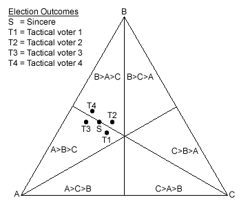
First consider a ranked ballot election in which three candidates A, B and C stand and the eight voters cast their sincere preferences without truncation as shown in the table below. The election outcome is a tie for first place as A and B both have the same number of first, second and third preferences. With fewer first and second preferences, candidate C is ranked in last place. Note that this outcome is independent of the preference weightings used in this election.

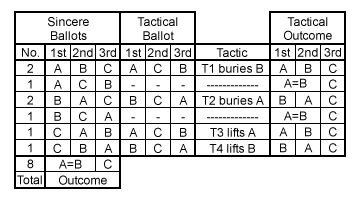
However, if tactical voter T1 "buries" B by casting A>C>B instead of A>B>C, then T1 breaks the critical tie in favour of their most preferred option A. Similarly, tactical voter T2 could bury A and achieve a tactical win for B since T2 prefers B over A. Supporters of the losing candidate C also have tactical options if they are prepared to "compromise" and raise their second choice to first preference. If T3 ranks A or T4 "lifts" B above their optimal choice C, then their sincere second preference scores a tactical win over their least preferred one without relying on a tie-break randomly producing the same outcome. Hence, GV does not satisfy the No-Favourite-Betrayal criteria as a more preferred election outcome is achieved by this betrayal of their first choice candidate.

These tactical shifts are listed in the table above and the resultant election outcomes are shown in the map above. Note that the shift from the sincere outcome (S) to any tactical outcome (T) is always parallel to the baseline for the unaltered preference. For example, T1 buries B by casting A>C>B instead of A>B>C. As the ranking of A is unchanged, points S and T1 on the map are equidistant from the baseline BC. However, given the preference swap between B and C, point T1 compared to point S is now closer to apex C and further from apex B thus placing it in the winning ranking region for A.

Comparison of Voting System Susceptibilities

The focus in the above example is only on one election profile and no particular voting system is identified. Continuing with three candidates and eight voters, each voter casts one out of six possible ranked ballots; namely, A>B>C, A>C>B, B>A>C, B>C>A, C>A>B or C>B>A. There are therefore six to the power eight or 1,679,616 permutations to consider. As it is unimportant as to which voter casts which ballot, the total number of different election profiles that could result from the election fortunately reduces to 1035. It must be noted that many different ranked ballot voter inputs produce identical candidate tallies. The number of such unique tally outcomes depends heavily on the weightings used by the specific voting system but is always much less than the number of election profiles.

The following analysis considers all these possible input profiles for four significant and key voting systems; namely, CHPV, the Borda Count, plurality and anti-plurality. The latter two methods are treated here as positional voting ones for comparison purposes. Also, to aid comparisons and map constructions, all four systems are normalised such that the first preference is worth 1-x, the second x and the third 0. While the tallies will differ between the actual and their equivalent voting systems, the rank ordering of the candidates remains identical. The four voting systems and their equivalent weightings are detailed below.

• Plurality with weightings (1,0,0) where x = 0
• CHPV with weightings (3/4,1/4,0) where x = 1/4
• Borda Count with weightings (2/3,1/3,0) where x = 1/3
• Anti-Plurality with weightings (1/2,1/2,0) where x = 1/2

Proceed to next page > Comparisons: Geometric Voting 10

Return to previous page > Comparisons: Geometric Voting 8